Linear Models (Again)
This lab script teaches the implementation and interpretation of the basic linear model by reference to Braithwaite’s (2006) analysis of the geographic spread of militarized interstate disputes. Students should read that article to understand the context of what we’re doing. This lab script will just implement one of their basic models and unpack its contents.
#          ___
#      _.-|   |          |\__/,|   (`\
#     {   |   |          |o o  |__ _) ) # not again...
#      "-.|___|        _.( T   )  `  /
#       .--'-`-.     _((_ `^--' /_<  \
#     .+|______|__.-||__)`-'(((/  (((/
#
# Lab 4b: Linear Models (Again)
If it’s not installed, install it.
library(tidyverse)
#> ── Attaching core tidyverse packages ──────────────────────── tidyverse 2.0.0 ──
#> ✔ dplyr     1.1.4     ✔ readr     2.1.4
#> ✔ forcats   1.0.0     ✔ stringr   1.5.0
#> ✔ ggplot2   3.5.2     ✔ tibble    3.3.0
#> ✔ lubridate 1.9.4     ✔ tidyr     1.3.0
#> ✔ purrr     1.1.0
#> ── Conflicts ────────────────────────────────────────── tidyverse_conflicts() ──
#> ✖ dplyr::filter() masks stats::filter()
#> ✖ dplyr::lag()    masks stats::lag()
#> ℹ Use the conflicted package (<http://conflicted.r-lib.org/>) to force all conflicts to become errors
library(stevethemes)
library(stevemisc)
#>
#> Attaching package: 'stevemisc'
#>
#> The following object is masked from 'package:lubridate':
#>
#>     dst
#>
#> The following object is masked from 'package:dplyr':
#>
#>     tbl_df
Load the data
This code aims to augment what students should’ve already learned in
the previous lesson.
I’ll be repeating myself because repetition will certainly help the
student’s learning, but I hope any terseness (for the moment) is met
with some understanding since it’s a fair bit of work to create new
lessons on the fly. No matter, I hope students have learned by now how
to read data from the internet. I’ve uploaded the data for this session
to Athena (in both forms) and to my website. You have two options here
if you’re going the route of my website. One is the Stata file and the
other is the R serialized data frame (.rds). Let’s go with the R
serialized data frame for this session. If you go this route, you have
to include url() in the readRDS() function. Observe:
Braith <- readRDS(url("https://svmiller.com/extdata/braithwaite2006gsmd.rds"))
# Braith <- haven::read_dta("https://svmiller.com/extdata/braithwaite2006gsmd.dta")
# ^ also works. You can also download a copy of the data fraom Athena.
This part won’t be super fun, but this is the price of doing business in this world. Ideally, you read the article in question to get an idea of what Alex is doing. Joshua Alley has these data in his Github repository of simple cross-sectional OLS data sets. The original data and analyses were conducted in Stata, so some forensics are necessary here based on the Stata .do file that Alex wrote. We’re going for a replication of Table II, so let’s identify what exactly he did and get a reduced version of the data based on Alex’ description and the Stata .do file. I’ll do it for you this session but, in the Master’s level, I’ll ask you to figure stuff out like this yourself. It’s good experience.
Before we begin, though, I welcome anyone in the class as we’re doing this to tell me what this article is about.
Briefly, we’re aiming to reproduce this model, presented below in Stata syntax.
# reg log_radius_area territory logsize host_mt host_for water cwpceyrs bord_vital host_resource if final_hostile>0, robust;
Okay, let’s look at our data…
Braith
#> # A tibble: 296 × 26
#>    dispnum dyadid ccode1 ccode2  year logcap_ratio allies joint_democ incidents
#>      <dbl>  <dbl>  <dbl>  <dbl> <dbl>        <dbl>  <dbl>       <dbl>     <dbl>
#>  1    4327  91093     91     93  2001        0.144      1           1         1
#>  2    4085 437475    437    475  1993        1.92       1           0         1
#>  3    4114 670679    670    679  1994        1.93       1           0         8
#>  4    4191 630640    630    640  1996        0.211      0           0         1
#>  5    4228 365700    365    700  1998        3.71       0           0         3
#>  6    4001 800811    800    811  1994        1.97       0           0        23
#>  7    4225 731740    731    740  1999        1.54       0           0         3
#>  8    4064 710713    710    713  1995        2.47       0           0        16
#>  9    4338 365373    365    373  1999        3.69       1           0         1
#> 10    4086 355705    355    705  1996        0.362      0           0         1
#> # ℹ 286 more rows
#> # ℹ 17 more variables: territory <dbl>, sdd <dbl>, radius <dbl>,
#> #   final_hostile <dbl>, jointsize <dbl>, log_radius_area <dbl>,
#> #   log_sdd_area <dbl>, pop_dense <dbl>, water <dbl>, logdurat <dbl>,
#> #   cwpceyrs <dbl>, host_mt <dbl>, host_for <dbl>, host_resource <dbl>,
#> #   bord_vital <dbl>, log_jointsize <dbl>, `_est_model1` <dbl>
names(Braith)
#>  [1] "dispnum"         "dyadid"          "ccode1"          "ccode2"
#>  [5] "year"            "logcap_ratio"    "allies"          "joint_democ"
#>  [9] "incidents"       "territory"       "sdd"             "radius"
#> [13] "final_hostile"   "jointsize"       "log_radius_area" "log_sdd_area"
#> [17] "pop_dense"       "water"           "logdurat"        "cwpceyrs"
#> [21] "host_mt"         "host_for"        "host_resource"   "bord_vital"
#> [25] "log_jointsize"   "_est_model1"
This is a good lesson for those of you who may have some experience with
Stata from another program. Stata will guess stuff on your behalf. R
won’t. In this case, Stata can infer you meant log_jointsize in the
data when you asked for logsize. R 100% won’t do that for you. Beyond
that, reducing the raw data to a simple form for the sake of the
analysis isn’t that hard.
Braith %>%
  filter(final_hostile > 0) %>%
  select(log_radius_area, territory, log_jointsize,
         host_for, host_mt, water, cwpceyrs, bord_vital,
           host_resource) -> Data

Data
#> # A tibble: 296 × 9
#>    log_radius_area territory log_jointsize host_for host_mt water cwpceyrs
#>              <dbl>     <dbl>         <dbl>    <dbl>   <dbl> <dbl>    <dbl>
#>  1            4.36         0          12.4   0         0        0        0
#>  2            4.36         0          17.1   0         0        0        1
#>  3           10.7          1          14.7   0.0686   44.2      0        4
#>  4            4.36         0          14.7   1.38     58.2      0        7
#>  5           10.2          0          16.7   0        13.6      0        0
#>  6           11.4          1          13.5  34.7      27.8      0        6
#>  7            4.36         0          13.1   0         0        0        0
#>  8           13.5          1          16.1  22.5      56.0      0        0
#>  9            4.36         0          16.6  10.9      49.2      0        5
#> 10            4.36         0          14.9   1.16      7.71     0        5
#> # ℹ 286 more rows
#> # ℹ 2 more variables: bord_vital <dbl>, host_resource <dbl>
How did we do?
summary(M1 <- lm(log_radius_area ~ territory + host_resource + host_mt +
                   host_for + water + bord_vital + log_jointsize + cwpceyrs,
                 data = Data))
#>
#> Call:
#> lm(formula = log_radius_area ~ territory + host_resource + host_mt +
#>     host_for + water + bord_vital + log_jointsize + cwpceyrs,
#>     data = Data)
#>
#> Residuals:
#>    Min     1Q Median     3Q    Max
#> -6.192 -2.479 -1.190  2.768  9.494
#>
#> Coefficients:
#>                Estimate Std. Error t value Pr(>|t|)
#> (Intercept)    4.496996   1.948533   2.308 0.021717 *
#> territory      1.624430   0.412026   3.943 0.000101 ***
#> host_resource  0.984149   0.431537   2.281 0.023307 *
#> host_mt        0.025871   0.007775   3.328 0.000990 ***
#> host_for      -0.012035   0.007177  -1.677 0.094620 .
#> water         -0.600507   0.558129  -1.076 0.282863
#> bord_vital    -0.809148   0.407514  -1.986 0.048032 *
#> log_jointsize  0.135650   0.125150   1.084 0.279319
#> cwpceyrs      -0.040498   0.012939  -3.130 0.001928 **
#> ---
#> Signif. codes:  0 '***' 0.001 '**' 0.01 '*' 0.05 '.' 0.1 ' ' 1
#>
#> Residual standard error: 3.395 on 287 degrees of freedom
#> Multiple R-squared:  0.1448, Adjusted R-squared:  0.121
#> F-statistic: 6.074 on 8 and 287 DF,  p-value: 3.154e-07
Got it. Don’t worry about the difference in the test statistics as we’re not going with robust standard errors for the sake of this exrecise. I explain a bit about what those are here.
Unpacking the Model Output
R presents a summary of the residuals at the top, though our eyes should
go right to the coefficients first (the extent to which we are
interested in hypothesis-testing). In Alex’ case, he’s interested in
explaining the geographic spread of militarized interstate disputes
through a variety of factors. He’s interested first, it seems, in the
pernicious effect of territorial disputes. He hypothesizes that disputes
over the allocation of territory are more likely to be dispersed over a
geographic area than disputes over any other issues. The coefficient for
that territory variable is 1.624. The standard error is .412. Dividing
the coefficient over the standard error for 287 degrees of freedom
results in a test statistic of 3.943. If there were truly no difference
between disputes over territory and disputes over any other issue, the
probability we observed what we observed is .000101. Thus, we reject the
null hypothesis as incompatible with the data we observed and suggest
Alex’ hypothesized relationship is closer to what it truly is. Since the
dependent variable is log-transformed, you’ll want to think of some
creative ways to express this relationship. I discuss these
here.
For example:
- Toggling a dispute from over some other issue to the allocation of
territory multiplies the geographic spread (as measured in the
radius from the center of the dispute to its furthest incident) by
exp(1.624)(about 5.075). - Toggling a dispute from over some other issue to the allocation of
territory results in a
(exp(1.624) - 1)*100(about 407.33) percent increase in the geographic spread of the dispute (as measured by the radius from the center of the dispute to its furthest incident).
Since the coefficient isn’t close to 0, I would advise against using the
rule of thumb of multiplying the coefficient by 100. You could, however,
do that with the forest variable (host_for). Alex doesn’t argue this
point with any obvious emphasis, but his treatment on pp. 510-11 implies
that forest would be impassable terrain. This should constrain the
spread of the dispute and a negative relationship should emerge. He
measures this by the percentage of the territory that is covered in
forest. The coefficient for this is -.012 and is significant at the .10
level in this model without robust standard errors. Thus, you can
communicate the relative change, percentage change, and percentage
change approximations by the following ways:
exp(-0.012035)-1       # relative change
#> [1] -0.01196287
(exp(-0.012035)-1)*100 # percentage change
#> [1] -1.196287
-0.012035*100          # percentage change approximation
#> [1] -1.2035
You can do something similar for the mountainous terrain variable, even as this has a different effect than the one hypothesized by Alex.
exp(0.025871)-1       # relative change
#> [1] 0.02620856
(exp(0.025871)-1)*100 # percentage change
#> [1] 2.620856
0.025871*100          # percentage change approximation
#> [1] 2.5871
If this is a bit much for you at this level, that’s cool too. You can just note what’s significant and in what direction and say something like “a one-unit change in the percentage of the territory that is covered in mountains coincides with an estimated change of .025 in the logged value of the radius between the center of the dispute to the furthest incident.” I’d be remiss, though, if I didn’t give you things to consider.
We should also make an obligatory reference to the stuff included at the bottom of the output. Namely, the adjusted R-squared suggests the model accounts for about 12% of the variation in geographic spread. We’ve also comfortably beat the mean-only model (see: the F-stat).
Again, with the Diagnostics
Let’s inspect the model output as we did in the previous lesson. Remember: the fitted-residual plot is the most “bang for your buck” linear model diagnostic. It’s where you should start.
plot(M1, which = 1)
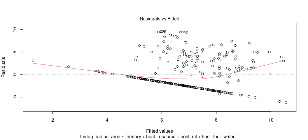
Oh boy… that’s not good. Let’s pretty it up bit, just for presentation
and added exposure to the augment() function in {broom}.
broom::augment(M1) %>%
  ggplot(.,aes(.fitted, .resid)) +
  geom_point(pch = 21) +
  theme_steve(style='generic') +
  geom_hline(yintercept = 0, linetype="dashed", color="red") +
  geom_smooth(method = "loess")
#> `geom_smooth()` using formula = 'y ~ x'
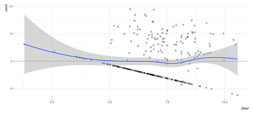
Remember what you should want to see in a fitted-residual plot. Know this isn’t it. That said, here’s what you can discern this is telling you and what it might mean for things you’d want to do with your model.
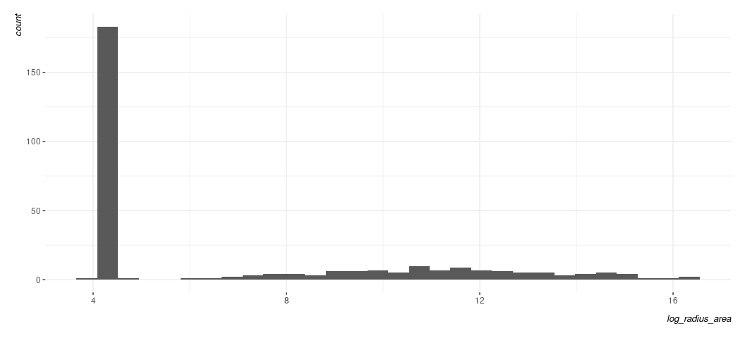
The first thing that grabs your attention is the clear line. Generally, a line like this of any kind in your fitted-residual plot is suggesting some kind of discrete pattern in the DV. Let’s see this for ourselves.
Data %>% ggplot(.,aes(log_radius_area)) +
  geom_histogram() +
  theme_steve(style='generic')
#> `stat_bin()` using `bins = 30`. Pick better value with `binwidth`.
Data %>% arrange(log_radius_area)
#> # A tibble: 296 × 9
#>    log_radius_area territory log_jointsize host_for host_mt water cwpceyrs
#>              <dbl>     <dbl>         <dbl>    <dbl>   <dbl> <dbl>    <dbl>
#>  1            3.83         1          11.8    75.1    47.0      0        2
#>  2            4.36         0          12.4     0       0        0        0
#>  3            4.36         0          17.1     0       0        0        1
#>  4            4.36         0          14.7     1.38   58.2      0        7
#>  5            4.36         0          13.1     0       0        0        0
#>  6            4.36         0          16.6    10.9    49.2      0        5
#>  7            4.36         0          14.9     1.16    7.71     0        5
#>  8            4.36         0          14.7     0       8.60     0        0
#>  9            4.36         0          12.7    34.0    49.8      1        1
#> 10            4.36         0          13.8    86.8     4.70     0        0
#> # ℹ 286 more rows
#> # ℹ 2 more variables: bord_vital <dbl>, host_resource <dbl>
When you see something like this, it’s suggesting you have some kind of “hurdle” component to the data-generating process. There is a separate process that determines that big bar you see and then a separate one determining the variation in the flatter distribution to the right of it. Braithwaite’s third footnote is pointing to his 2005 data article in International Interactions that might provide more context for why this value of 4.363605 occurs so much in his data. I do not at all expect you to know exactly what to do under these circumstances. That said, here’s about what I’d expect you to say: “the fitted-residual plot suggests a clear discrete pattern in the DV and the histogram suggests two separate data-generating processes. Both strongly imply the linear model is a questionable fit for the data.”
The second thing that grabs your attention (maybe?) is the disagreement
between the LOESS smoother and the flat line at 0. I don’t know if it’s
no. 2, but it’s what we’ll talk about next. When you see something like
this, it’s suggesting some kind of non-linear relationship in the data.
It comes with three major caveats though. The first is that the LOESS
smoother will always come off the line at 0 near the tails of the
fitted-residual plot. Thus, we really shouldn’t say something with any
authority yet. The second is that we obviously have the discrete
clumping we noted above. That might be an important part of this. The
third is that we 100% won’t know where until we looked at something a
bit more informative. linloess_plot() in {stevemisc} will do this.
linloess_plot(M1, pch=21) +
  theme_steve(style='generic')
#> Warning: attributes are not identical across measure variables; they will be
#> dropped
#> `geom_smooth()` using formula = 'y ~ x'
#> `geom_smooth()` using formula = 'y ~ x'
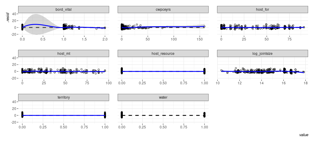
Binary IVs will never be the issue here. It’s the “vital border” variable that looks like it has some weirdness. Based on what I remember of Starr (2002) and how Alex describes this on p. 514, it would suggest that the 0s are probably a distinct phenomenon that should be focused on in some detail. Beyond that, it really seems like the fitted-residual plot’s LOESS smoother is really just drawing attention to the “hurdle” component of the DV.
The third thing you can tell from the fitted-residual plot is that the variance of the residuals are clearly fanning out as the fitted values increase. That’s as tell-tale a sign of heteroskedasticity as you’re going to see. It’s also why Alex estimated this model with robust standard errors. If I remember Stata correctly, this is type “HC1”.
lmtest::coeftest(M1,  sandwich::vcovHC(M1,type='HC1'))
#>
#> t test of coefficients:
#>
#>                 Estimate Std. Error t value  Pr(>|t|)
#> (Intercept)    4.4969959  1.6694475  2.6937 0.0074823 **
#> territory      1.6244297  0.4240554  3.8307 0.0001570 ***
#> host_resource  0.9841490  0.4425418  2.2239 0.0269364 *
#> host_mt        0.0258709  0.0072926  3.5475 0.0004540 ***
#> host_for      -0.0120354  0.0067672 -1.7785 0.0763824 .
#> water         -0.6005071  0.5610364 -1.0704 0.2853596
#> bord_vital    -0.8091477  0.3978571 -2.0338 0.0428950 *
#> log_jointsize  0.1356500  0.1122895  1.2080 0.2280269
#> cwpceyrs      -0.0404980  0.0103090 -3.9284 0.0001072 ***
#> ---
#> Signif. codes:  0 '***' 0.001 '**' 0.01 '*' 0.05 '.' 0.1 ' ' 1
I don’t expect you to know what this does, but I’ve pointed you in the direction of what this does on my blog. Don’t sweat those details now. Just know it’s what a lot of practitioners do in the presence of non-constant error variance (heteroskedasticity).
Finally, we can check for whether the residuals are normally distributed. This assumption has no bearing for our test statistics or our line of best fit, but it’s nice to estimate a model that can reasonably fit the data.
plot(M1, which=2)
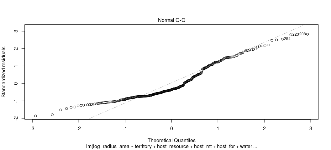
rd_plot(M1) + theme_steve(style='generic')
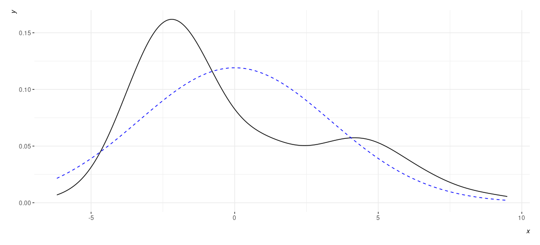
Again, a plot like this is wanting to alert us to the “hurdle” component of the DV. Rather than have normally distributed residuals, or something reasonably approximating it, we have two such peaks in our data. Non-normally distributed residuals strongly imply a non-normally distributed DV. We already knew we had that in this case.